Analysis Solution

The Analysis Document

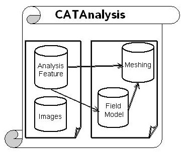
All Analysis data are stored inside the Analysis document. The extension of this document is "CATAnalysis". The data are stored in different containers.

The figure shows the contents of the CATAnalysis document in term of containers. All are created at the document initialization.

1. The "Analysis Feature" container groups the Specifications. It is based on features and literals in order to capture as much as possible the user's design intent. After, the Spec objects build an analysis model supported by finite element entities by using standard physical type description.
2. The "Field Model" container groups the concrete classes that define the view of the physics based on finite element entities.
3. The "Meshing" container is the result view of the mesh specifications. It groups concrete classes.
4. The "Images" container groups the Specifications that define the display of the analysis model. The Images container allows the physical types to be displayed once the are defined on finite element entities.

[Top]

Analysis Features

The Analysis features are the support for the specifications of the user. They support the V5 basic behaviors (Copy/Paste, update, navigation, selection, etc.).

[Top]

The End User View

The figure below shows a typical CATIA V5 work session within the Structural Analysis application. This Analysis document contains a reference to a design document (in this case, a Part document) on which a stress analysis is computed. This feature tree summarizes the different kinds of analysis features that are manipulated by the user interface. This same structure is used in order to scan the model when programming. What is the role of the different Analysis feature objects:

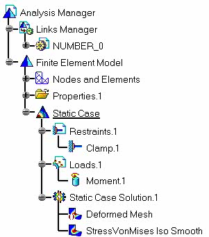An Analysis model is made of some different features. The Analysis Manager is the root feature that manages: The Links Manager role is to keep the link to the referenced design document. It can be a Part for single part analysis, a Product for analysis of a design assembly or other external documents. It is here a rod Part The Finite Element Model is dedicated to the discretization (meshing global and local specifications) and idealization (behavior of the part as physical properties). By default it contains a meshing set called Nodes and Elements, a property set, a material set, and an axis set. Relative to a Finite Element Model, some Analysis Cases are created in order to group all kinds of external data applied on the idealization. (In this case, Boundaries, Loads and the solution set that will give access to all the physical data that can be computed by the solver.) The Analysis Case is defined for a given solver and for a specific computation. (In this case, static linear.) It is made of Analysis Sets that groups some Analysis Entities, which represent some physical preprocessing actions applied to the design. (For this example, apply a clamp or a momentum to B-rep elements of the part.) In order to have the result visualization, images appear in the tree. They are connected in the tree under the set that provides the values for the display. In this example, they are connected under the Static Case Solution.1.

[Top]

Programming with Analysis Features

By default, after the document initialization, the Analysis document contains the Analysis Manager, the Links Manager and one FEM model. The following graph explains the dependency between the features and the interfaces implemented on the features.

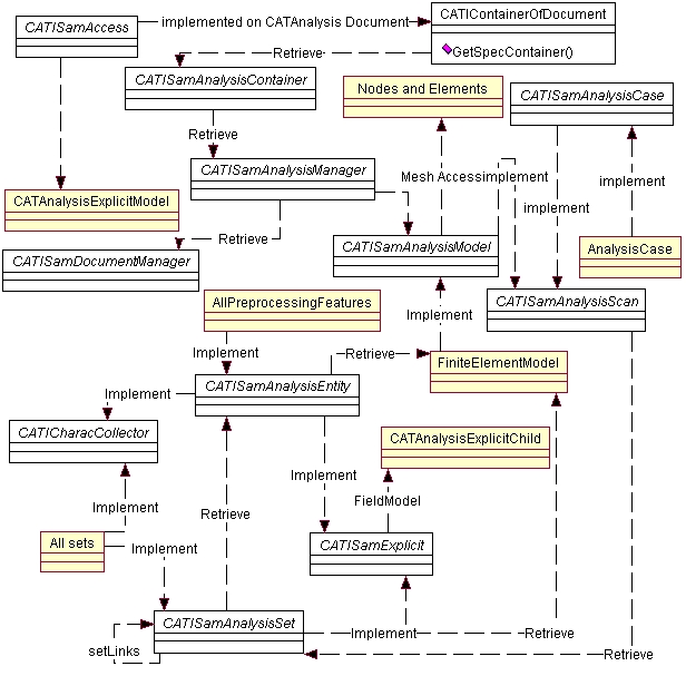
From a pointer to the Analysis document, query a pointer to the CATISamAccess interface in order to retrieve the root container thanks to the GetSpecContainer method. This enables you to access the features. From the CATIContainer pointer returned, query a pointer to the CATISamAnalysisContainer interface.

From this CATISamAnalysisContainer pointer, you can use the GetAnalysisManager method to retrieve the CATISamAnalysisManager or query a pointer to the CATISamAnalysisModelFactory interface that manages all the methods for the analysis feature creation.

The CATISamAnalysisManager interface provides the methods to access the CATISamDocumentManager in order to manage the document linked to the current Analysis document, and access the different CATISamAnalysisModel methods implemented by the feature set called FEMModel.

The CATISamAnalysisModel interface provides the methods to access the analysis cases that apply to it using a pointer to CATISamAnalysisCase interface. Both implement the CATISamAnalysisScan interface that allows the analysis sets that make up the analysis model to be retrieved as pointers to the CATISamAnalysisSet interface. At the document initialization, an empty analysis model is created and contains the following sets:

• MeshSet for Meshing definition (This set implements also the CATIMSHMeshManager interface in order to access the meshing information)
• MaterialSet for Material definition
• AxisSet for local axes definition
• PropertySet for physical properties definition.

By default for structural analysis and static linear displacement computation, the Analysis Case is made of the following sets:

• RestraintSet for boundary's definition
• LoadSet for external load definition
• StaticSet for the computation management. This set is dedicated to an ELFINI computation and will support its implementations of CATIEdit for interactive edition capability, CATIBuild for launching the solver, and CATICharacCollector for extracting the available solver results.

By default for structural analysis and modal computation, the Analysis Case is made of the following sets:

• RestraintSet for boundary's definition
• MassSet for "non-structural" mass definition
• DymaniqueSet for the computation management. This set is dedicated to an ELFINI computation and will support its implementations of CATIEdit for interactive edition capability, CATIBuild for launching the solver, and CATICharacCollector for extracting the available solver results.

CATISamAnalysisSet provides methods to create and access the analysis entities that make up the analysis set. These entities implement CATISamAnalysisEntity.

Any analysis entity is made of Physical data that implement CATISamBasicComponent (that accesses the physical data under literal [1] format in order to take benefit of ) and implement by itself CATISamAnalysisSupport (that manages the selection of finite element entities based on geometrical data). From the analysis entity, you can use the CATISamAnalysisEntity interface to retrieve its basic components or use CATISamAnalysisSupport for its analysis support by querying a pointer to the appropriate interface.

[Top]

Interfaces for Analysis Features

This part will describe the recommanded way of using CAA interfaces on Analysis features.

• CATIEdit is used for the edition of a feature from tree selection. If your feature is build by derivation of "AnalysisSet" or "AnalysisEntity" and made of Basic components, a default implementation is provided. This default implementation manages the model and the Visual Basic of the object. This implementation can be overloaded.
• CATIBuild  is used for updating a feature. It is recommended not to implement this interface and to prefer the implementation of CATISamExplicitation.
• CATI3DGeoVisu is used to associate a 3D rep to a feature. By default it is implemented for all analysis features. To customize an analysis entity visualization implement CATISamEntityVisu and let the default adapter managing the connection to the visualization manager, pre-highlight of the support, and impact between entities in the feature tree.
•  

[Top]

Field Model

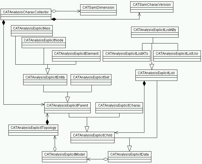
This model is designed in order to support the finite element view of the specification. Specification means pre-processing and post-processing model and data access. The field model is made of concrete classes that must not be derived and of a dictionary that defines the physical types list and category, and the rules for the model as well. Note that when manipulating those classes, you are using a class close to an handler and not a pointer. The pointer of an explicit class is typed as CATSamExplicitPtr define. To store locally arrays of explicit objects, use the CATAnalysisExplicitListUsr or arrays of CATSamExplicitPtr.

The main field model components are:

• CATAnalysisExplicitModel that supports the general access.
• CATAnalysisExplicitRulesData that supports the physical type definition and the rules for the model.
• CATAnalysisExplicitSet is the image in the field model of an analysis set, analysis model or analysis case Spec Object.
• CATAnalysisExplicitEntity is the image in the field model of an analysis Entity Spec Object.
• CATAnalysisExplicitNode is the image in the field model of a meshing node.
• CATAnalysisExplicitElement is the image in the field model of a meshing element.
• CATAnalysisExplicitCharac is the physical data that support the numerical values once they are converted from the specification to its finite element support. The kinds of values that are supported are char, short, int, float, CATMathComplexf, double, CATMathComplex or CATSamExplicitPtr. The values are returned as cont pointer to an array stored in the data-member of the characteristic or as a duplication of the array.
• CATAnalysisCharacCollector manage the characteristics obtained by combining the information of basics characteristics over several entities. It support also the data returned by computation for post-processing. This object is defined by a Physical Type, a version, and a position.

  In order to build a collector characteristic, you must use the following methods in this order:

  • SetContext to retrieve the Explicit object parent of the CharacCollector.
  • SetDefinition to initialize its physical type, version, position and occurrences parameters.
  • SetNbEntities to initialize the number of entities that may have values (currently, it is the number of nodes or element of the model).
  • SetEntities to initialize the entities that will have values.
  • SetDimension to initialize the dimensions parameters.
  • SetValues to initialize the values. The kinds of values that are supported are the same as for the CATAnalysisExplicitCharac object.
  • SetPositionUVWCoordinates, SetCoordinateSystems (optionally) to initialize specific position to define where the values are applied.

A physical type is defined by the CATSamPhysicalType typedef. It can be considered as an enumeration that can be converted into an identifier during programming, or into a string for printing. All methods required to manipulate them are defined by using the CATAnalysisExplicitRulesData class with the help of CATAnalysisExplicitDefinition enumerates.

A version is defined by the CATSamCharacVersion object. This object is built according to the information list:

A Position is a CATString instance. It defines the positions on which field data entities can be applied. Existing position list is:

• NONE for general data like set parameters.
• NODE for data attached to nodes.
• DOF for data attached to degrees of freedom (See CATSamDof for their description).
• ELEMENT for data attached to finite elements.
• EDGE for data attached to finite element edges.
• FACE for data attached to finite element faces.
• CENTER for data attached to the center of finite elements.
• NODE_OF_ELEMENT for data attached to the nodes of finite elements.
• GAUSS for data attached to the gauss points of finite elements.

The general graph of the model can be summarized in the following image. It shows the principal object used for programming and the way they are implemented inside the field model. The instantiation of the CATAnalysisExplicitModel launches in memory the dictionary (an external file called "mechanical") that provides the list of physical types and the rules for the object design and relationship. According to this file, the Structural Analysis defines a default format for linear mechanical analysis.

To access the data inside the CATAnalysisCharacCollector object, use the CATSamDimension object. Some additional information are describe in the FAQ Quick Reference.

The following diagram summarize the relationships of the field model objects:

[Top]

Physical Types for Structural Analysis

The Sets Definition

For programming help the following array shows the correspondences between a feature late type, it's name is displayed on the screen (NLS) and the Physical type associated. This physical type is also the one of the Set that represent the feature in the field model.

[Top]

The Preprocessing Entities Definition

They are described in the following reference [2].

[Top]

Local Axis Definition

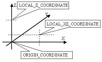
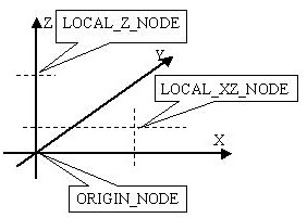
Six kinds of local axes can be defined in the field model. They can be identified by explicit coordinates or nodes in order to define rectangular, cylindrical, and spherical axes as follows:

Physical Type list:

• AXIS_RECTANGULAR_3D_NODE
• AXIS_RECTANGULAR_3D_COORDINATE
• AXIS_CYLINDRICAL_3D_NODE
• AXIS_CYLINDRICAL_3D_COORDINATE
• AXIS_SPHERICAL_3D_NODE
• AXIS_SPHERICAL_3D_COORDINATE

With Associated Characteristics:

AXIS_XXX_3D_COORDINATE	AXIS_XXX_3D_NODE

[Top]

Getting Access to the Physical Types (CharacCollector) Available for an Analysis Feature

The access the different physical types of an existing feature can be retrieved by using implement the CATICharacCollector interface. For all the Preprocessing features (sets and entities) an implementation is provided. By using the reference [3], see how to extract this physics.

[Top]

Meshing Model

The meshing model is stored in the meshing container and contains the finite element discretisation data.

[Top]

Accessing the Meshing Model

The access to the meshing container is done by using the general feature tree. The feature set "Nodes and Elements" implements an interface that allow to work with the feature object included in the meshing container: CATIMSHMeshManager. This feature is build by derivation of the AnalysisSet startup, So it supports all the CATISamAnalysisSet behavior.

From this interface, you can retrieve:

• The Mesh Part Management. This interface should be used to access all data associated to a Mesh Part, such as global and local mesh specifications or geometry to be meshed (supports). A Mesh Part is an Analysis Set which has some specific attributes (global specifications and supports and can contain Analysis Entities which represent local mesh specifications. Associated to each Mesh Part, there is a mesher which is called to check the supports and to build the mesh by using the CATIMSHMesh interface.
• The Meshing container CATIMSHMesh interface that allows you to create/scan CATMSHNode, CATMSHElement, and access CATIMSHConnectivity. For the meshing modeler point of view, a CATMSHElement is defined at least by its connectivity (geometrical shape) and linked nodes (CATMSHNode object).
• The manager of Associativity with design data. CATIMSHAssociativity interface to retrieve the finite element entities that are linked to geometrical entities.
• The Connectivity's information (Geometrical definition of the finite element, integration scheme, etc.).

[Top]

The Meshing Model Connectivity's

The following reference article shows the ways the connectivity's are provided by the meshing model. It defines the way to scan faces, edges and nodes of the elements.

[Top]

Integrating the Meshing Inside the Field Model

The CATMSHNode and CATMSHElement are represented inside the field model as Explicit Entities. The entity for CATMSHNode has a physical type NODE. For CATMSHElement, the physical type is defined as ELEMENT_"Elementtype"_Dimension_Geometry. This offers the capability to complete the geometrical information by adding some physical data and to make a distinction between a physical BAR (ELEMENT_BAR_3D_BAR2) and a BEAM (ELEMENT_BEAM_3D_BAR2) defined on the same BAR connectivity. For programming facilities, the specific classes CATAnalysisExplicitNode and CATAnalysisExplicitElement may be used.

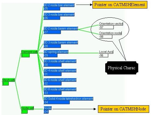
For example, a large number of the connections defined for the Structural Assembly application are for a meshing point of view multi-nodes elements defined with a SPIDER connectivity. For the field model, the physic types of the elements can be:

• ELEMENT_CONSTRAINT_3D_BAR
• ELEMENT_CONSTRAINT_3D_BEAM
• ELEMENT_CONSTRAINT_3D_MEAN
• ELEMENT_CONSTRAINT_3D_JOIN

All the preprocessing data are applied to this explicit entities.

[Top]

From Features to Field Model Generation

The interfaces for this are CATISamExplicit and CATISamExplicitation.

• CATISamExplicit role is to manage the Field model object(s) associated to a feature.
• CATISamExplicitation role is to generate the Field model object(s).

According to the figure presenting the analysis features:

• By default, all the analysis sets implement the CATISamExplicit and CATISamExplicitation interfaces. The implementations create a single CATAnalysisExplicitSet. To do this, use CATSamCatalogFactory::SetPhysicalType  to valuate on the feature StartUp an attribute named "PhysicalType" with an appropriated string defined in the field model dictionary. The explicit Object is created when the Feature set is associated to its parent by the use of the AddSet method of the CATISamAnalysisScan interface. This interface is implemented on AnalysisModel, AnalysisCase and AnalysisSet (to build Set of Sets). This set will be retrieved using the GetExplicitObject method. The interface CATISamExplicitation  have to be re-implemented if its default behavior is not satisfactory. For example, you can re-implement it in order to have one ExplicitSet associated to some ExplicitCharac that represent some additional physics (for example, the variable data that manages the different steps associated to a set).

• The same behavior can be applied en entities. All the analysis entities provided by Dassault Systèmes products implement the CATISamExplicit interface that create a single explicit entity CATAnalysisExplicitEntity. This entity is created in the field model when the AddEntity method of the CATISamAnalysisSet is called. After its build, the entity will be completed with some CATAnalysisExplicitCharac and will be applied to the corresponding finite element entities.

• By association of this Explicit Object, the CATICharacCollector interface is implemented on each analysis set and analysis entity provided by Dassault Systèmes products and the CATAnalysisCharacCollector will be attached under the corresponding object in the field model. It is called the parent of the CharacCollector.

General Update scheme.

The following graph show how the analysis features are plug together in order to have a convenient update behavior.

[Top]

Example for Existing Preprocessing Set and Entities

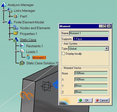This preprocessing feature applies a momentum on a face of a design "Part". The specifications are made up of a vector definition (Basic Component) called "Moment Vector" (that can be expressed according to a particular axis system) and a face support (that can be a multi-selection of B-rep elements of the Part). This feature implements the CATISamEntityVisu interface in order to display the 3D representation at the right location (highlighted on the face). The CATISamExplicitation interface will generate in the field model a distribution of forces applied onto nodes linked with the support as displayed in the next image

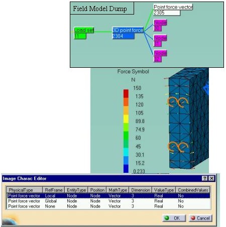The dump of the field model shows the Load set associated with the LOAD feature, and the Explicit entity that represents a 3D nodal force made up of one explicit characteristic that manages one vector per node on which the force entity is computed by the distribution. The charac-collector implemented on this feature will retrieve the Physical type “Point force vector” associated with the versions “Local”, “Global” or “None” according to the reference frame in which the vector is expressed and a position “Node” (that is, the only position to express the vectors).

[Top]

Programming with Field Model Objects.

This chapter describes the different ways of designing a field model associated to a preprocessing entity. Typical model is made of an entity, parent of some characteristics and applied on finite element support. Some capabilities can be used to distribute values according to where they are applied. This model structures are used by the preprocessing feature provided by DASSAULT SYSTEMES applications and insure the generation of charac-collectors. If you need to complete the model, you may generate structures that respects those rules.

To understand more, you have to refer to :

• The different ApplyTo methods of the explicit entity. The most general method is described here:

• The object that allow to manage values on according to the apply of an entity is the CATAnalysisExplicitCharac. For this refer to the SetDefinition Method, or the CreateCharac Method with full definition parameters. The recommendation for proper initialization of a characteristic definition, is to use the CATAnalysisExplicitRulesData -> GetPhysicalTypeMathematicalInfo that will initialize all the parameters. Then for a iValueType defined as default as float, you can change it as double, complex float or complex, double. You can change the iRepeat and the iDistributionMode.

Some examples of model definition:

Model Definition	How it will be collected ?
	Each node has the same force vector applied on it. This force is defined by a vector expressed in a global reference frame. In this case, the number of values of POINT FORCE is 3.
	Each node has the different force vector applied on it. This force is defined by a vector expressed in a global reference frame. n this case, the number of values of POINT FORCE is 6.
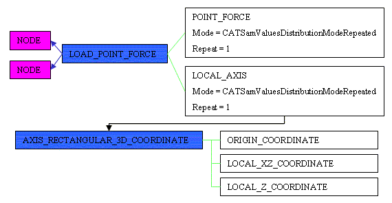	Each node has the same force vector applied on it. This force is defined by a vector expressed in one single local reference frame. In this case, the number of values of POINT FORCE is 3.
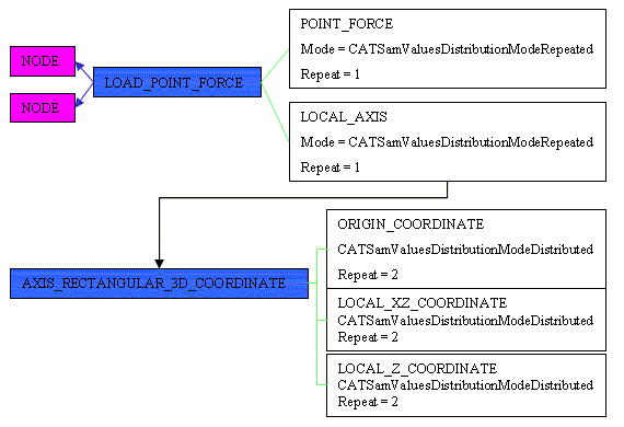	Each node has the same force vector applied on it. This force is defined by a vector expressed in two different local reference frame. In this case, the number of values of POINT FORCE is 3. the number of values for each of the characteristics of the Local axis is 6. Note that another way of building the same model is to define the local axis with a distributed mode, and a repeat set to 2. Then, the local axis references to reference frames with standard definition (Repeated mode, and number of repeat set to one).
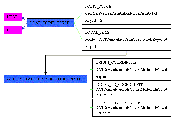	Each node has the different force vector applied on it. This force is defined by a vector expressed in two different local reference frame. In this case, the number of values of POINT FORCE is 6. the number of values for each of the characteristics of the Local axis is 6. Note that another way of building the same model is to define the local axis with a distributed mode, and a repeat set to 2. Then, the local axis references to reference frames with standard definition (Repeated mode, and number of repeat set to one).
	Objective is to assign a temperature distribution at finite elements. In Addition, we want to have a gradient between upper and lower face. Each element receives twice a temperature, (by making twice the apply) and the usage of CATSamApplyQualifier specify witch value is associated to each face of the element.
	Objective is to assign a nodal forces at the node of the finite elements. In this case, apply is done on elements. in order to have variable forces for the each elements. The size of values for the force characteristic is the somme of the number of nodes for each elements applied on. This model can be also completed with local axes. Note that: CATSamValuesDistributionModeRepeatedOnVertexOfElements means that values are distributed on each Vertex Nodes of the elements, and repeated on each element. CATSamValuesDistributionModeDistributedOnVertexOfElements means that values are distributed on each vertex node of the elements and on each element. In this scenario, values are collected at the elements and the position of the charac-collector is NODE_OF_ELEMENT.

As other example, to assign the same loading force at a specific same position to all elements of a loading entity:

Note that in this case the loading condition is applied on a ONE dimension element, in this case set up the dimension of the position to 1. When using GetPositionUVWCoordinates, only the U will be set Up (consider you are in the local reference frame of the finite element. To do the same on a 2D element set up the dimension of the position characteristic to 2 and enter couple of values as values of POSITIONS. In this case, UV coordinates will be set up.

[Top]

Example for Existing Solution Sets

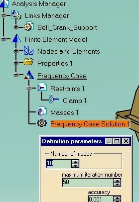
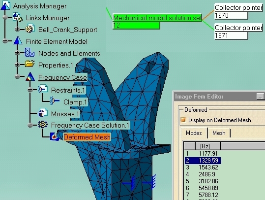
This set is defined as the output set of Cases. All the implementations presented are related to the CATIA-ELFINI © solver. The following example is relevant to Frequency Solution. From a feature view, the set have some parameters and a link to an external file (called external storage) that is of the ELFINI© proprietary format. By implementing the CATICharacCollector interface, this format is translated into the standard Charac-Collector format. The associated field model is made up of an explicit set (with the physical type "MECHANICAL_MODAL") to which are attached the Charac-Collector(s) that the solver can retrieve inside its database or compute dynamically.

[Top]

Implementing New features

For an example of implementation and more details on the methods to implement, see the reference [4].

[Top]

In Short

This document presented some of the high level concepts of CATIA Analysis Interfaces. The other technical articles and the use cases will demonstrate how to use them with concrete scenario.

[Top]

References

History

Copyright © 2000, Dassault Systèmes. All rights reserved.